Here's an example.

 

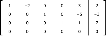
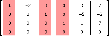
To see where to go from here, let's look at a concrete example, using the augmented matrix above.

At the bottom is a row of zeroes, which translates into the equation "0 = 0". This is always true, so it contributes no information about the solutions of the system. You can just ignore this row.

Here's a summary of the complete process.

To solve a linear system when its augmented matrix is in reduced row-echelon form

1. If there's a leading 1 in the last column, stop: there is no solution.
2. Otherwise, identify the leading variables and the free variables. Assign parameter values to the free variables.
3. Translate the non-zero rows of the matrix back into equations.
4. Solve each equation for its leading variable in terms of the parameters.

When you apply row operations to an augmented matrix, you generally want to end up with a matrix in a very specific form. Some terminology: the first non-zero number in any row of your augmented matrix is called the leading entry, or pivot entry for that row.

A matrix is in reduced row-echelon form when

any rows of all zeroes are at the bottom

the leading entry in any other row is a 1 (called a leading 1, or pivot 1)

each leading 1 is further to the right than any leading 1's above it

any column with a leading 1 has zeroes in the rest of that column.

Using row operations to transform a matrix into reduced row-echelon form is called row-reducing the matrix (to reduced row-echelon form). Row reduction is a very common process in linear algebra used for many processes besides solving linear systems. For how to do it, see the learning object How to Row Reduce a Matrix

Once your augmented matrix has been transformed into reduced row-echelon form, there's a systematic way to solve the linear system. Each row of your new matrix corresponds to an equation, and the new system of equations has the same solutions as the old one.

Now translate the non-zero rows of the matrix back into equations:

x1 – 2x2 + 3x5 = 2,   or   x1 = 2 + 2s – 3t
x3 – 5x5 = -3,   or   x3 = –3 +5t
x4 + x5 = 7,   or   x4 = 7 - t .

The full solution to the system is then

x1 =2 + 2s – 3t
x2 = s
x3 = -3 + 5t            for parameters s and t.
x4 =7 – t
x5 = t

In other words, the parameters s and t can take on any values, but once you choose those values, the values of the other variables are completely determined.

Notice that a linear system may have

• no solution (in which case it's said to be inconsistent),
• a single solution (with no parameters, called a unique solution) or
• infinitely many solutions (i.e. a solution with one or more parameters, each of which can take on any real number as value).

A system with 5 equations in three variables has the unique solution x = 1, y = 2 and z = 3. What does the reduced row-echelon form of its augmented matrix look like?

Can a linear system with more variables than equations have a unique solution? Why or why not?

Suppose first that your reduced augmented matrix has a "bad row" - a string of zeroes with a 1 in the very last column. The bad row translates into the equation "0 = 1". This is impossible - no values of the variables can satisfy this equation. Your system has no solution and no further calculation will change that, so you stop.

All the information about the solutions of the system is in the remaining rows. The next step is to identify the leading variables (those corresponding to a column with a leading 1) and the free variables (the rest). (The free variables are called free because they can take on any value; none of the equations relates any of them to each other.)

For this system, the leading variables are x1, x3 and x4 and the free variables are x2 and x5. Assign arbitrary parameter variables to these free variables to indicate their freedom: set set x2 = s and x5 = t.